Rendering in 3D Gaussian Splatting
This blogpost is a web version of my notes for my “WebGPU 3D Gaussian Splatting” renderer. I’ve focused only on the forward path, especially what to do after we already have the covariance matrix. There are 2 main approaches here:
- Use the larger eigenvalue to find a square around the Gaussian’s mean. Most often used with a tiled renderer.
- Use eigenvectors to find the axis of the ellipsis. Place vertices on these axes.
I’ve described the math for both approaches.
These are my notes, the notation is going to be sketchy.
Our main sources will be:
- “3D Gaussian Splatting for Real-Time Radiance Field Rendering” by Bernhard Kerbl, Georgios Kopanas, Thomas Leimkühler, and George Drettakis.
- “EWA Volume Splatting” by Matthias Zwicker, Hanspeter Pfister, Jeroen van Baar, and Markus Gross.
Goal
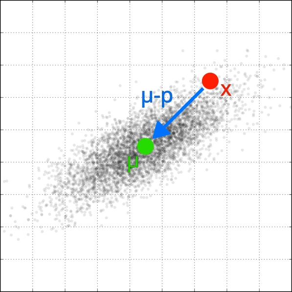
Each Gaussian’s transform is described using position, rotation, and scale. When projected onto a screen, it will have the shape of an ellipsis. You might remember from the principal component analysis that the eigenvectors of the covariance matrix form the axis of this ellipsis. Our goal is to get the image space covariance matrix.
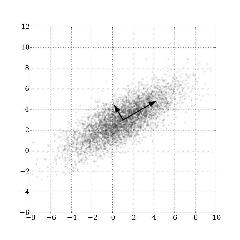
Principal component analysis of a multivariate Gaussian distribution. The vectors shown are the eigenvectors of the covariance matrix.
Covariance 3D
Each Gaussian has a scale (vector ) and rotation (quaternion with real part and imaginary parts ). We need transformation matrices for both.
Scale:
Rotation (assuming unit quaternion):
From the definition of covariance matrix you might notice that is proportional to the sample covariance matrix of the dataset X. If the mean is 0, the sum becomes a dot product. Like matrix multiplication. How does covariance change if we have 2 transformation matrices? Let , the combined transformation. Then the covariance of this 3D Gaussian is . From the properties of the transposition, we know that . Then . The scale matrix is diagonal, so . The transposition of the rotation matrix is equal to its inverse. This might come in handy during debugging. Be prepared for left/right-handedness issues.
Covariance is the parameter of the Gaussian. It’s better if you don’t think of “calculating the covariance matrix given scale and rotation”. Instead, the Gaussian is parametrized by the covariance. So it happens that gives a covariance matrix. Not sure if this makes sense, but I found this to be clearer. Additionally, backpropagation is easier with rotation and scale instead of the raw matrix. Covariance matrices have to be symmetric and positive semi-definite.
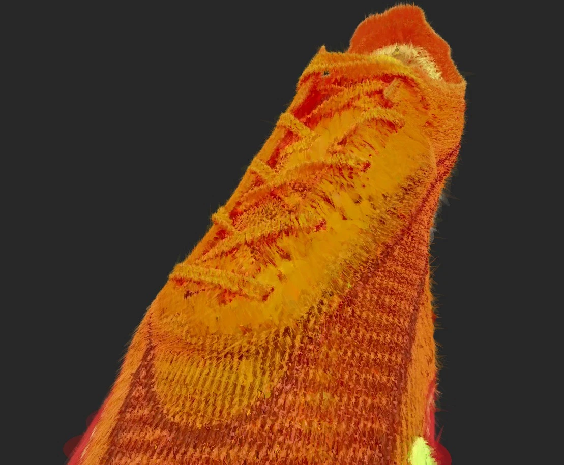
Model rendered with the inverted rotation matrix.
Covariance 2D
In 3D graphics, to project a vertex into a clip space we multiply its position by view and projection matrices. Let denote our view matrix. For Gaussians we will use the following Jacobian instead of a projection matrix:
- p - position of the Gaussian in world space.
- t - position of the Gaussian in view space.
Check the explanation for the Jacobian in “EWA Volume Splatting”, section 4.4 “The Projective Transformation”. From what I understand, the mapping to perspective space can introduce perspective distortion. Depending on where on screen the Gaussian is rendered, it would have different size? The paper mentions that this mapping is not affine. I.e. it does not preserve parallelism. Use ray space instead. Find more details in:
- “EWA Volume Splatting”,
- “[Concept summary] 3D Gaussian and 2D projection” (Google translated from Korean),
- “Fundamentals of Texture Mapping and Image Warping” by Paul S. Heckbert (section 3.5.5).
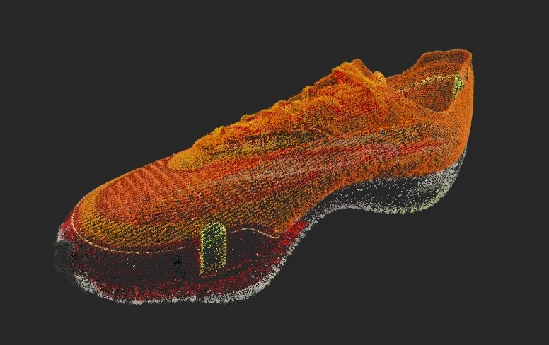
Rendered model with projection matrix used instead of Jacobian.
The values for focal distance depend on the camera settings. Based on the perspective matrix values and geometric definition of tangent:
const focalX = projectionMat[0] * viewport.width * 0.5;
const focalY = projectionMat[5] * viewport.height * 0.5;
The perspective matrix calculation only takes half of the provided field of view. Hence multiplication by 0.5. Depending on our coordinate system, you might have to transpose this matrix.
With this, we can calculate :
This uses the same trick as we have used for calculations.
We are only interested in the 2D projection of the Gaussian (we discard depth). Get the 2D variance matrix from the by removing the third, and fourth rows and columns:
If the determinant of the cov2d is ≤ 0 then the shape would be a parabola or a hyperbola instead of an ellipsis.
At this point, the reference implementation adds to the cov2d. It’s done to ensure that the matrix is invertible. You can find the detailed explanation in AI葵’s “Gaussian Splatting Notes (WIP)”.
Calculating eigenvalues
I recommend reading the Eigenvalues_and_eigenvectors article on Wikipedia. The “Matrix examples” section has nice examples.
Let’s calculate the eigenvalues. To make notation simpler, I’ve assigned a letter to each element of the 2D matrix cov2d.
when (calculating the roots of the quadratic equation):
Remember that (. Might make the implementation easier.
The and (the eigenvalues) are the radii of the projected ellipsis along major and minor axes. Since the value for the square root is always >1 (at least in our case), then > . You would expect this from the ellipsis projection.
Right now we have 2 options. We can either get the eigenvectors to derive vertex positions. This is not what the “3D Gaussian Splatting” paper did. They’ve collected all the Gaussians for each tile of their tiled renderer using conservative approximation. We will derive both solutions, starting with the one used in the paper.
Method 1: Project Gaussian to a square
Calculate tiles
The Gaussian distribution has a value even at infinity. This means that every Gaussian affects every pixel. Most of them with negligible results. We want to know which closest tiles it affects the most. Look at the 1D Gaussian distribution, and find radius “r” so that contains most of the area. For normal distribution with :
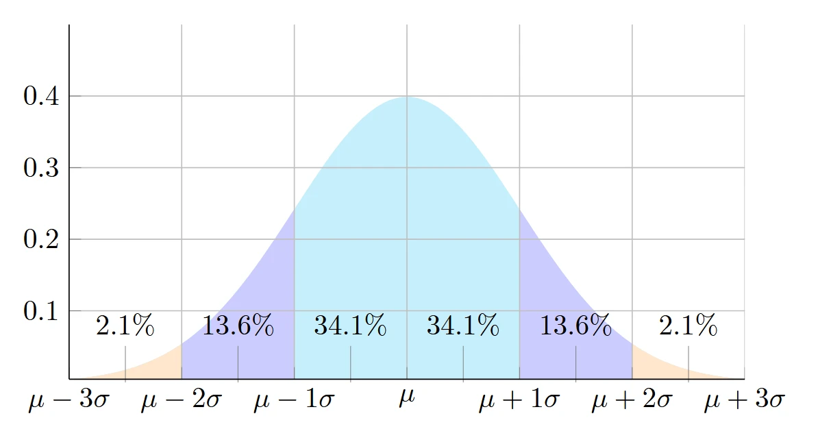
Normal distribution with . Percentage numbers for relative area between each standard deviation.
For example, if you picked , then the integral has a value of ~0.9973. Such an approximation has an error of ~0.27%. As you might suspect, the variance will affect the calculations. We end up with . Sigma is a variance of the Gaussian. For us, it’s (where has a bigger value).
let radius = ceil(3.0 * sqrt(max(lambda1, lambda2)));
The radius is in pixels. We also have the Gaussian’s position projected into an image space. Every tile inside the radius around the projected position is affected by the Gaussian. To map it to tiles, we calculate the affected square: projectedPosition.xy +- radius.xy.
let projPos = mvpMatrix * gaussianSplatPositions[idx];
// (we can also cull the Gaussian here if we want)
projPos /= projPos.w; // perspective divide
let projPosPx = ndc2px(projPos.xy, viewportSize);

// https://github.com/graphdeco-inria/diff-gaussian-rasterization/blob/59f5f77e3ddbac3ed9db93ec2cfe99ed6c5d121d/cuda_rasterizer/auxiliary.h#L46
let BLOCK_X = 16, BLOCK_Y = 16; // tile sizes
let blockSize = vec2<i32>(BLOCK_X, BLOCK_Y);
// block count for x,y axes
let grid = (viewportSize.xy + blockSize.xy - 1) / blockSize.xy;
let rectMin = vec2<i32>(
  min(grid.x, max(0, (int)((projPosPx.x - radius) / BLOCK_X))),
  min(grid.y, max(0, (int)((projPosPx.y - radius) / BLOCK_Y)))
);
let rectMax = vec2<i32>(
  min(grid.x, max(0, (int)((projPosPx.x + radius + BLOCK_X - 1) / BLOCK_X))),
  min(grid.y, max(0, (int)((projPosPx.y + radius + BLOCK_Y - 1) / BLOCK_Y)))
);
With this, we know which tiles are affected by each Gaussian.
Depth sorting
For each tile, we will need its Gaussians sorted by the distance to the camera (closest first). For sorting on the GPU, Radix sort is popular, but Bitonic sort is much easier to implement. On the CPU, you can use your language’s built-in sort for a terrible performance. Or Counting sort for something 6+ times better (according to my app’s profiler).
Gaussian’s value at pixel
You might know the general form of the Gaussian distribution:
“EWA Volume Splatting” provides a function (eq. 9) for the density of an elliptical Gaussian centered at a point with a variance matrix :
The above formula depends on the dimensionality. Only the changes. Here, “d” denotes dimensionality (2 in our case).
In our case, V=cov2d matrix. We need its determinant () and inverse :
In “EWA Volume Splatting”, the inverse of the variance matrix is called the conic matrix. You might have seen this word used as a variable name.
Projected 3D Gaussian. (“p” in “EWA Volume Splatting” notation) is the projected mean of the Gaussian. The “x” is the center of an example pixel.
We will now look at . Let’s and:
After matrix multiplication and a dot product:
We can then calculate as an exponential falloff from the mean point of the Gaussian at the pixel p. Multiply the result by the Gaussian’s innate opacity (learned during the training). The was removed (?). Your trained model file will not display correctly if you add it back in.
Blending
Rendering transparent objects is always done starting from the closest ones. Blend N Gaussians for a pixel using the following formula (eq. 3 from “3D Gaussian Splatting” paper):
- - RGB color of the i-th Gaussian.
- - a combination of Gaussian’s innate transparency at the current pixel wrt. its projected position and the opacity learned during the training.
This equation can be rephrased as:
- The closest Gaussian writes its color . Let’s say that , then we write .
- Next closest Gaussian (let’s say ) blends its color: .
- Third closest Gaussian (let’s say ) blends its color: .
Once the first Gaussian has written color with , the subsequent Gaussians can only affect the remaining 0.3 of the color. The 2nd Gaussian had . It writes its color with effective opacity . The 3rd Gaussian can only affect of the output color. This repeats till we have gone through all Gaussians that touch this pixel. Writing to is a convenient way to carry over alpha calculations to the next Gaussians.
At some point, the impact of subsequent Gaussians will be negligible. From the paper:
“When we reach a target saturation of 𝛼 in a pixel, the corresponding thread stops. At regular intervals, threads in a tile are queried and the processing of the entire tile terminates when all pixels have saturated (i.e., 𝛼 goes to 1). (…) During rasterization, the saturation of 𝛼 is the only stopping criterion. In contrast to previous work, we do not limit the number of blended primitives that receive gradient updates. We enforce this property to allow our approach to handle scenes with an arbitrary, varying depth complexity and accurately learn them, without having to resort to scene-specific hyperparameter tuning”.
Code
Below is the corresponding code from the original repo. I’ve changed the formatting, and substituted comments to correlate the code with the equations above.
float2 xy = collected_xy[j];
float2 d = { xy.x - pixf.x, xy.y - pixf.y }; // (x-p), in my equations it's [x_0, y_0]
// Values for conic. Assigning the values that I have used:
// a = con_o.x
// b = con_o.y
// c = con_o.z
float4 con_o = collected_conic_opacity[j];
float power = -0.5f * (con_o.x * d.x * d.x + con_o.z * d.y * d.y) - con_o.y * d.x * d.y;
if (power > 0.0f)
    continue;

// con_o.w is the Gaussians' alpha learned during the training.
// alpha is the opacity if there was no blending
float alpha = min(0.99f, con_o.w * exp(power));
if (alpha < 1.0f / 255.0f) // skip if alpha too small
    continue;

// Blending accumulation. T is from the previous iteration
float test_T = T * (1 - alpha);
if (test_T < 0.0001f) {
    done = true;
    continue;
}

// Eq. (3) from 3D Gaussian splatting paper.
for (int ch = 0; ch < CHANNELS; ch++) {
    // Gaussian's learned color * opacity
    C[ch] += features[collected_id[j] * CHANNELS + ch] * alpha * T;
}

T = test_T;// blending accumulation to reuse during next loop
We have now seen how to render the Gaussian by projecting it as a square. This technique is often used in tiled (compute shader-based) renderers. Or, we can use the eigenvectors to calculate vertex positions in the rendered pipeline.
Method 2: Calculate eigenvectors
Sorting and the index buffer
We will be blending the Gaussians into the framebuffer. Firstly, sort them based on the depth (closest to the camera first). A popular way is to use an index buffer. Render each Gaussian as a quad (2 triangles). With triangle list topology, each triangle has 3 indices. Total 6 indices (vertex shader invocations) per Gaussian. In the vertex shader, we need to know both the splat index and which vertex of the splat we are working with. Steps:
- Sort the Gaussians and write the Gaussian’s index into a u32[] buffer of size
BYTES_U32 * splatCount. - Create a buffer for “unrolled” indices of size
BYTES_U32 * splatCount * 6. - Fill the “unrolled” based on the sorted Gaussians (see code below).
- Read splatIdx and vertexInSplatIdx inside vertex shader:
@builtin(vertex_index) in_vertex_index: u32or gl_VertexID depending on the shading language.let splatIdx = in_vertex_index / 6u;let vertexInSplatIdx = in_vertex_index % 6u;
Code for “unrolling” the sorted splatIds to encode both splatIdx and vertexInSplatIdx:
for (let i = 0; i < splatCount; i++) {
  const splatIdx = sortedSplatIndices[i];
  // write 6 consecutive values
  unrolledSplatIndices[i * 6 + 0] = splatIdx * 6 + 0;
  unrolledSplatIndices[i * 6 + 1] = splatIdx * 6 + 1;
  unrolledSplatIndices[i * 6 + 2] = splatIdx * 6 + 2;
  unrolledSplatIndices[i * 6 + 3] = splatIdx * 6 + 3;
  unrolledSplatIndices[i * 6 + 4] = splatIdx * 6 + 4;
  unrolledSplatIndices[i * 6 + 5] = splatIdx * 6 + 5;
}
Afterward, bind the index buffer and draw splatCount * 6 vertices.
Vertex shader - eigenvectors
We will continue from the point where we have calculated and . Remember this image from the beginning of the article?
Principal component analysis of a multivariate Gaussian distribution. The vectors shown are the eigenvectors of the covariance matrix.
Continuing with the eigenvalues and eigenvectors article, calculate the eigenvector for :
Expressing in terms of , so we have that we can normalize:
The eigenvector:
We have the values for . We will treat this as a normalized vector - the directions of the ellipsis major/minor axis. In code, we can substitute any value for , as we will normalize it anyway. You can also solve:
let diagonalVector = normalize(vec2(1, (-a+b+lambda1) / (b-c+lambda1)));
let diagonalVectorOther = vec2(diagonalVector.y, -diagonalVector.x);
let majorAxis = 3.0 * sqrt(lambda1) * diagonalVector;
let minorAxis = 3.0 * sqrt(lambda2) * diagonalVectorOther;
cov2d is a symmetric matrix and , so the eigenvectors are orthogonal. We scale respective axis vectors by radii using (just as in the “tiled” renderer) . This works but may lead to problems at oblique angles. Most implementations clamp it to 1024.
I’ve seen some implementations multiply by instead. Either I’ve missed something, or they (if I had to guess) forgot to divide and by 2.
The fixes result in the following implementation:
let majorAxis = min(3.0 * sqrt(lambda1), 1024) * diagonalVector;
let minorAxis = min(3.0 * sqrt(lambda2), 1024) * diagonalVectorOther;
// depends on which quad vertex you calculate
let quadOffset = vec2(-1., -1.);// or (-1., 1.), or (1., 1.), or (1., -1.)
projPos.xy += quadOffset.x * majorAxis / viewportSize.xy
            + quadOffset.y * minorAxis / viewportSize.xy;
result.position = vec4<f32>(projPos.xy, 0.0, 1.0);
result.quadOffset = quadOffset;
Fragment shader
Full fragment shader at the end of this section. Whole 6 LOC.
Let’s imagine that our vertices produced a square. Then imagine our fragment shader draws a circle inside of this square (something like length(uv.xy - 0.5) < 1). This is exactly what we will do. With 2 modifications:
- Smudge a circle so it does not have hard edges. Cause you know, it’s Gaussian.
- Use Gaussian’s color and opacity for blending.
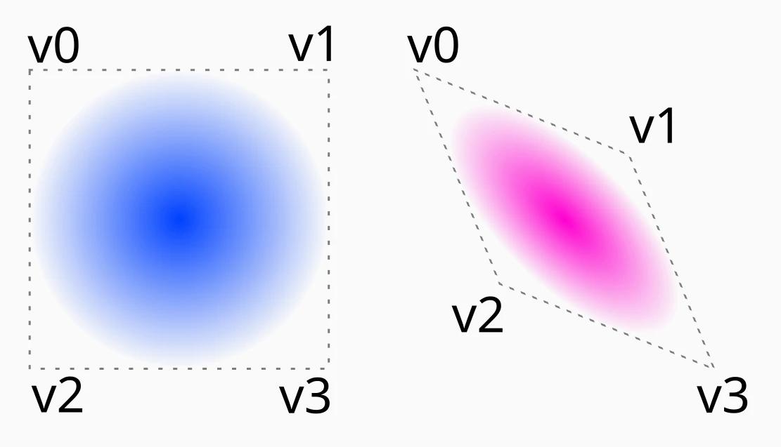
Circle gradient when vertices form a square and rhombus.
To solve the first issue, we go back to “EWA Volume Splatting”, section 6 “Implementation”:
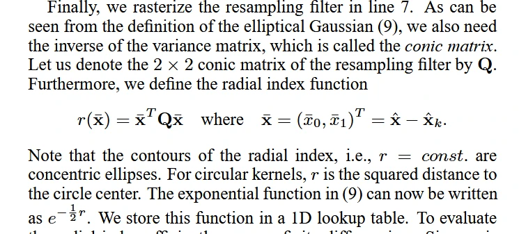
Derivation of . From “EWA Volume Splatting”.
The equation (9) is the one we have seen during tile renderer discussions:
I’m not sure about the derivation of . It’s the Gaussian’s opacity based on the pixel’s distance from the center. The Gaussian’s color also includes transparency. This means color blending. That’s the reason why we have sorted the Gaussians before the rendering.
Blending settings
In graphic API we do not have access to colors written by previous invocations of the fragment shader. Instead, use the following blend functions:
 color: {
  srcFactor: "one-minus-dst-alpha",
  dstFactor: "one",
  operation: "add",
},
alpha: {
  srcFactor: "one-minus-dst-alpha",
  dstFactor: "one",
  operation: "add",
},
They are equivalent to what we have discussed for the tiled renderer. Make sure that the clearColor for the framebuffer sets the alpha component to 0.
Final fragment shader
The whole fragment shader in WGSL:
@fragment
fn fs_main(fragIn: VertexOutput) -> @location(0) vec4<f32> {
  let r = dot(fragIn.quadOffset, fragIn.quadOffset);
  if (r > 1.0){ discard; } // circle

  let splatOpacity = fragIn.splatColor.w;
  let Gv = exp(-0.5 * r);
  let a = Gv * splatOpacity;
  return vec4(a * fragIn.splatColor.rgb, a);
}
You might notice that both rendering methods calculated either or . In truth, both are exchangeable if you know how to derive them and adjust for vertex positions.
References
- “3D Gaussian Splatting for Real-Time Radiance Field Rendering” by Bernhard Kerbl, Georgios Kopanas, Thomas Leimkühler, and George Drettakis.
- “EWA Volume Splatting” by Matthias Zwicker, Hanspeter Pfister, Jeroen van Baar, and Markus Gross.
- “First time streaming in the U.S. (Talking about Gaussian Splatting cuda code)” by AI葵(AI Aoi). Has English subtitles.
- “Combination of Multivariate Gaussian Distributions through Error Ellipses” by Clayton V. Deutsch and Oktay Erten.
- “(Concept summary) 3D Gaussian and 2D projection” (Google translated from Korean).